Caret, nproc and naivebayes • naivebayes

1) Introduction

The naive_bayes() function, a powerful tool for classification, is readily accessible through the highly regarded Caret package. Additionally, it can be utilized seamlessly via the nproc package, providing users with alternative options. This concise documentation aims to demonstrate the basic usage of the naive_bayes() function in both the Caret and nproc packages.

2) Naive Bayes in Caret

The first part showcases how to train a Naive Bayes model using the naive_bayes() function within the caret interface in R. It provides an example of how to prepare the data, train the Naive Bayes model, and perform classification using the trained model. This section focuses on the core steps of training a Naive Bayes model and utilizing it for classification tasks.

The second part demonstrates the process of defining a tuning grid, performing resampling, and finding the “optimal” Naive Bayes model using the caret package in R. It outlines how to define a grid of tuning parameters, train multiple models with different parameter combinations, and select the best-performing model based on resampling techniques. This section emphasizes the importance of tuning the Naive Bayes model to achieve better performance and provides insights into the parameter selection process.

By combining these two sections, users can gain a comprehensive understanding of how to train and optimize Naive Bayes models using the naive_bayes() function within the caret interface in R.

2.1) Model Training with Caret

The model is trained using the caret::train() function, specifying "naive_bayes" as the method and setting usepoisson to TRUE to handle the count variable.

After training the model, classification can be performed by using the trained model to predict the class labels. Additionally, the model provides posterior probabilities, which can be obtained for further analysis.

If needed, the code allows accessing the underlying naive_bayes object, providing access to additional information and functionalities of the Naive Bayes model.

Overall, the code demonstrates the process of training a Naive Bayes model, performing classification, and accessing the model object for further analysis using the caret interface in R.

library(caret, quietly = TRUE)
library(naivebayes)

## naivebayes 1.0.0 loaded

## For more information please visit:

## https://majkamichal.github.io/naivebayes/

# Load the iris dataset
data(iris)

# Prepare the data
new <- iris[-c(1,2,3)]
set.seed(1)
new$Discrete <- sample(LETTERS[1:3], nrow(new), TRUE) 
set.seed(1)
new$Counts <- c(rpois(50, 1), rpois(50, 2), rpois(50, 10)) 


# Train the Naive Bayes model with the Caret package
naive_bayes_via_caret <- train(Species ~ ., 
                               data = new, 
                               method = "naive_bayes", 
                               usepoisson = TRUE)

## Print the trained model
# naive_bayes_via_caret

# Perform classification
head(predict(naive_bayes_via_caret, newdata = new))

## [1] setosa setosa setosa setosa setosa setosa
## Levels: setosa versicolor virginica

# Get posterior probabilities
head(predict(naive_bayes_via_caret, newdata = new, type = "prob"))

##      setosa   versicolor    virginica
## 1 1.0000000 2.004949e-08 9.549385e-14
## 2 1.0000000 4.242500e-08 3.229798e-13
## 3 1.0000000 2.512936e-08 1.566929e-13
## 4 0.9999999 5.203335e-08 5.710476e-13
## 5 1.0000000 2.004949e-08 9.549385e-14
## 6 0.9999514 4.860925e-05 4.128918e-10

# Access the underlying naive_bayes object
nb_object <- naive_bayes_via_caret$finalModel
class(nb_object)

## [1] "naive_bayes"

# nb_object

2.2) Parameter Tuning with Caret

First, a tuning grid is defined using the expand.grid() function, which specifies different combinations of tuning parameters for the Naive Bayes model.

Then, the Naive Bayes model is fitted with parameter tuning using the caret::train() function. The tuneGrid argument is used to provide the defined tuning grid. The resulting model is stored in the naive_bayes_via_caret2 object.

To view the selected tuning parameters, you can access naive_bayes_via_caret2$finalModel$tuneValue. If you uncomment the respective line of code, you can also view the final Naive Bayes model itself.

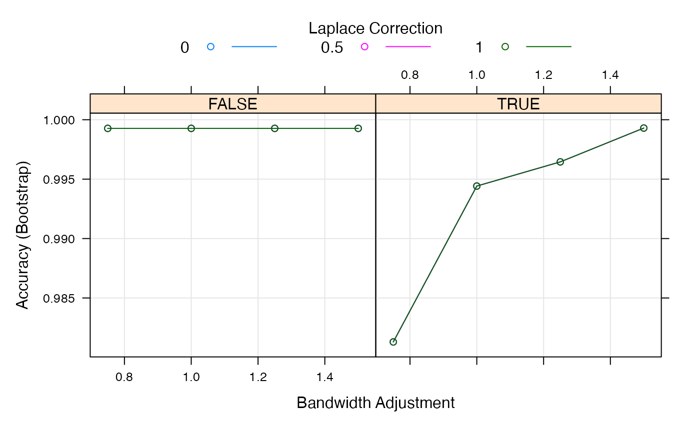
The tuning process can be visualized using the generic plot() function, which provides insights into the performance of different parameter combinations.

Finally, the trained model is used to perform classification on new data by using the predict() function. The class labels of the new data can be obtained with predict(naive_bayes_via_caret2, newdata = new).

# Define tuning grid 
nb_grid <- expand.grid(usekernel = c(TRUE, FALSE),
                       laplace = c(0, 0.5, 1), 
                       adjust = c(0.75, 1, 1.25, 1.5))

# Fit the Naive Bayes model with parameter tuning
set.seed(2550)
naive_bayes_via_caret2 <- train(Species ~ ., 
                                data = new, 
                                method = "naive_bayes",
                                usepoisson = TRUE,
                                tuneGrid = nb_grid)

# View the selected tuning parameters
naive_bayes_via_caret2$finalModel$tuneValue

##    laplace usekernel adjust
## 16       0      TRUE    1.5

## View the final naive_bayes model
# naive_bayes_via_caret2$finalModel

# Visualize the tuning process
plot(naive_bayes_via_caret2)

# Perform classification 
head(predict(naive_bayes_via_caret2, newdata = new))

## [1] setosa setosa setosa setosa setosa setosa
## Levels: setosa versicolor virginica

Overall, the code showcases the steps involved in defining a tuning grid, performing model training with parameter tuning, visualizing the tuning process, and applying the trained model for classification using the Naive Bayes algorithm within the caret package in R.

3) Naive Bayes in nproc

The nproc package provides Neyman-Pearson (NP) classification algorithms and NP receiver operating characteristic (NP-ROC) curves, and it can be used in conjunction with the naivebayes package. By incorporating the naivebayes package within the NP classification framework, users can leverage the power of the naive Bayes algorithm for binary classification tasks while controlling type I and type II errors effectively. This integration allows practitioners to apply the NP paradigm to the naive Bayes classifier and enhance its performance in various application domains.

# Example usage with nproc and naivebayes packages

# install.packages("nproc")
library(nproc)
library(naivebayes)

# Simulate data
set.seed(2550)
n <- 1000
x <- matrix(rnorm(n * 2), n, 2)
c <- 1 + 3 * x[ ,1]
y <- rbinom(n, 1, 1 / (1 + exp(-c)))
xtest <- matrix(rnorm(n * 2), n, 2)
ctest <- 1 + 3 * xtest[,1]
ytest <- rbinom(n, 1, 1 / (1 + exp(-ctest)))


# Train Naive Bayes classifier such that the type I error alpha is no bigger than 5%
naive_bayes_via_nproc <- npc(x, y, method = "nb", alpha = 0.05)

## Recover the "naive_bayes" object
# naive_bayes_via_nproc$fits[[1]]$fit

# Classification
nb_pred <- predict(naive_bayes_via_nproc, xtest)

# head(nb_pred$pred.label)

# Obtain various measures
accuracy <- mean(nb_pred$pred.label == ytest)
ind0 <- which(ytest == 0)
ind1 <- which(ytest == 1)
typeI <- mean(nb_pred$pred.label[ind0] != ytest[ind0])  # type I error on test set
typeII <- mean(nb_pred$pred.label[ind1] != ytest[ind1]) # type II error on test set

cat(" Overall Accuracy: ",  accuracy,"\n",
    "Type I error:     ", typeI, "\n",
    "Type II error:    ", typeII, "\n")

##  Overall Accuracy:  0.689 
##  Type I error:      0.02590674 
##  Type II error:     0.490228

The provided code demonstrates the usage of the nproc and naivebayes packages in R.

First, the necessary packages are loaded. Then, synthetic data is generated using the set.seed() function to ensure reproducibility. The data consists of two independent variables (x) and a binary response variable (y). A test dataset (xtest) is also generated for evaluation.

Next, the naive Bayes classifier is applied using the npc() function from the nproc package, with the method set to "nb" for naive Bayes. The alpha parameter is set to 0.05, defining a desirable upper bound on type I error.

After training the classifier, predictions are made on the test dataset using the predict() function. The accuracy of the predictions is calculated by comparing the predicted labels (nb_pred$pred.label) with the true labels (ytest).

Additionally, type I and type II errors are computed by comparing the predicted labels with the true labels separately for class 0 and class 1 instances. The type I error corresponds to misclassifying class 0 observations as class 1, while the type II error represents misclassifying class 1 observations as class 0.

Finally, the overall accuracy, type I error, and type II error are printed to the console using the cat() function.

The code demonstrates how to leverage the nproc and naivebayes packages to apply the Neyman-Pearson classification paradigm¹ to the naive Bayes classifier and evaluate its performance in terms of accuracy and error rates.