Plot Method for naive_bayes Objects

Plot method for objects of class "naive_bayes" designed for a quick look at the class marginal distributions or class conditional distributions of predictor variables.

Usage

# S3 method for naive_bayes
plot(x, which = NULL, ask = FALSE, legend = TRUE,
  legend.box = FALSE, arg.num = list(), arg.cat = list(),
  prob = c("marginal", "conditional"), ...)

Arguments

x

object of class inheriting from "naive_bayes".

which

variables to be plotted (all by default). This can be any valid indexing vector or vector containing names of variables.

ask

logical; if TRUE, the user is asked before each plot, see par(ask=.).

legend

logical; if TRUE a legend will be be plotted.

legend.box

logical; if TRUE a box will be drawn around the legend.

arg.num

other parameters to be passed as a named list to matplot.

arg.cat

other parameters to be passed as a named list to mosaicplot.

prob

character; if "marginal" then marginal distributions of predictor variables for each class are visualised and if "conditional" then the class conditional distributions of predictor variables are depicted. By default, prob="marginal".

...

not used.

Details

Probabilities are visualised by matplot (for numeric (metric) predictors) and mosaicplot (for categorical predictors). In case of non parametric estimation of densities, the bandwidths are reported for each class. Nothing is returned. For numeric (metric) predictors position of the legend can be adjusted changed via arg.num(..., legend.position = "topright"). legend.position can be one of "topright" "topleft", "bottomright", "bottomleft". In order to adjust the legend size following argument can be used: arg.num(..., legend.cex = 0.9).

The parameter prob controls the kind of probabilities to be visualized for each individual predictor \(Xi\). It can take on two values:

• "marginal": \(P(Xi|class) * P(class)\)

• "conditional": \(P(Xi|class)\)

Author

Michal Majka, michalmajka@hotmail.com

See also

naive_bayes, predict.naive_bayes, %class%, tables, get_cond_dist

Examples

data(iris)
iris2 <- cbind(iris, New = sample(letters[1:3], 150, TRUE))

# Fit the model with custom prior probabilities
nb <- naive_bayes(Species ~ ., data = iris2, prior = c(0.1, 0.3, 0.6))

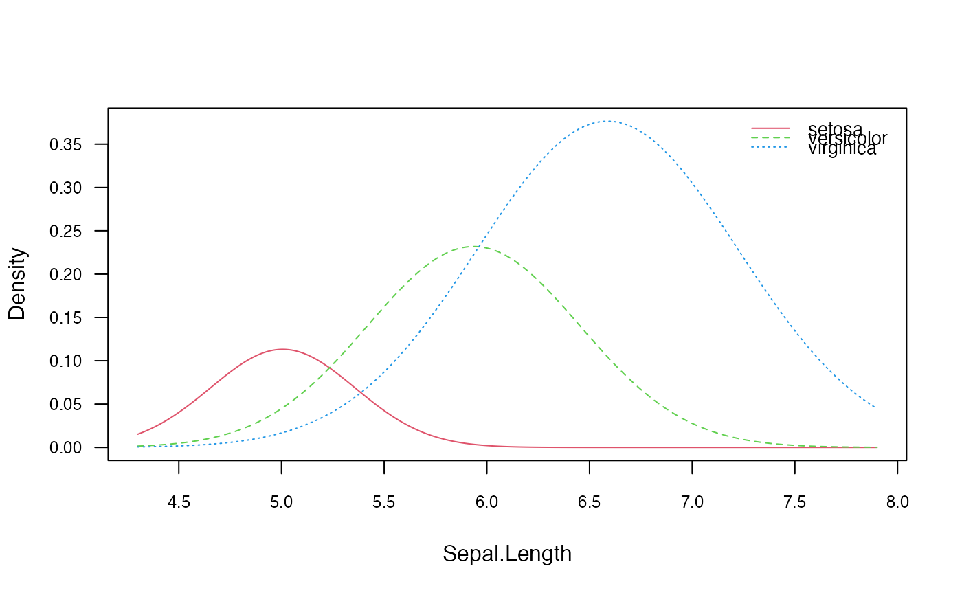
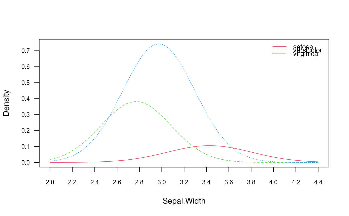
# Visualize marginal distributions of two predictors
plot(nb, which = c("Sepal.Width", "Sepal.Length"), ask = TRUE)



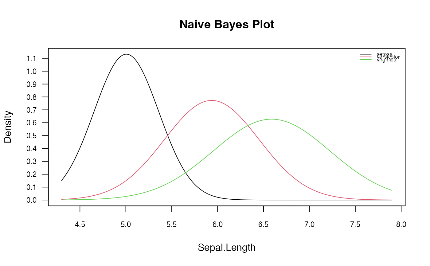
# Visualize class conditional distributions corresponding to the first predictor
# with customized settings
plot(nb, which = 1, ask = FALSE, prob = "conditional",
     arg.num = list(col = 1:3, lty = 1,
     main = "Naive Bayes Plot", legend.position = "topright",
     legend.cex = 0.55))


# Visualize class marginal distributions corresponding to the first predictor
# with customized settings
plot(nb, which = 1, ask = FALSE, prob = "marginal",
     arg.num = list(col = 1:3, lty = 1,
     main = "Naive Bayes Plot", legend.position = "topright",
     legend.cex = 0.55))


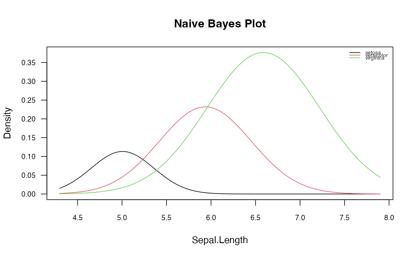
# Visualize class marginal distribution corresponding to the predictor "new"
# with custom colours
plot(nb, which = "New", arg.cat = list(color = gray.colors(3)))