Poisson Naive Bayes Classifier

poisson_naive_bayes is used to fit the Poisson Naive Bayes model in which all class conditional distributions are assumed to be Poisson and be independent.

Usage

poisson_naive_bayes(x, y, prior = NULL, laplace = 0, ...)

Arguments

x: numeric matrix with integer predictors (matrix or dgCMatrix from Matrix package).
y: class vector (character/factor/logical).
prior: vector with prior probabilities of the classes. If unspecified, the class proportions for the training set are used. If present, the probabilities should be specified in the order of the factor levels.
laplace: value used for Laplace smoothing (additive smoothing). Defaults to 0 (no Laplace smoothing).
...: not used.

Value

poisson_naive_bayes returns an object of class "poisson_naive_bayes" which is a list with following components:

data: list with two components: x (matrix with predictors) and y (class variable).
levels: character vector with values of the class variable.
laplace: amount of Laplace smoothing (additive smoothing).
params: matrix containing class conditional means.
prior: numeric vector with prior probabilities.
call: the call that produced this object.

Details

This is a specialized version of the Naive Bayes classifier, in which all features take on non-negative integers (numeric/integer) and class conditional probabilities are modelled with the Poisson distribution.

The Poisson Naive Bayes is available in both, naive_bayes and poisson_naive_bayes. The latter provides more efficient performance though. Faster calculation times come from restricting the data to an integer-valued matrix and taking advantage of linear algebra operations. Sparse matrices of class "dgCMatrix" (Matrix package) are supported in order to furthermore speed up calculation times.

The poisson_naive_bayes and naive_bayes() are equivalent when the latter is used with usepoisson = TRUE and usekernel = FALSE; and a matrix/data.frame contains only integer-valued columns.

The missing values (NAs) are omited during the estimation process. Also, the corresponding predict function excludes all NAs from the calculation of posterior probabilities (an informative warning is always given).

Note

When the parameter laplace is set to positive constant c then this amount is added to all counts. This leads to the ("global") Bayesian estimation with an improper prior. In each case, the estimate is the expected value of the posterior which is given by the gamma distribution with parameters: cell count + c and number of observations in the cell.

If in one cell there is a zero count and laplace = 0 then one pseudo-count is automatically to each such cell. This corresponds to the "local" Bayesian estimation with uniform prior.

Author

Michal Majka, michalmajka@hotmail.com

Examples

library(naivebayes)

### Simulate the data:
set.seed(1)
cols <- 10 ; rows <- 100
M <- matrix(rpois(rows * cols, lambda = 3), nrow = rows, ncol = cols)
y <- factor(sample(paste0("class", LETTERS[1:2]), rows, TRUE, prob = c(0.3,0.7)))
colnames(M) <- paste0("V", seq_len(ncol(M)))
laplace <- 0.5


### Train the Poisson Naive Bayes
pnb <- poisson_naive_bayes(x = M, y = y, laplace = laplace)
summary(pnb)
#> 
#> ============================= Poisson Naive Bayes ============================== 
#>  
#> - Call: poisson_naive_bayes(x = M, y = y, laplace = laplace) 
#> - Laplace: 0.5 
#> - Classes: 2 
#> - Samples: 100 
#> - Features: 10 
#> - Prior probabilities: 
#>     - classA: 0.28
#>     - classB: 0.72
#> 
#> -------------------------------------------------------------------------------- 

# Classification
head(predict(pnb, newdata = M, type = "class")) # head(pnb %class% M)
#> [1] classB classB classB classB classB classB
#> Levels: classA classB

# Posterior probabilities
head(predict(pnb, newdata = M, type = "prob")) # head(pnb %prob% M)
#>         classA    classB
#> [1,] 0.2796812 0.7203188
#> [2,] 0.1973988 0.8026012
#> [3,] 0.2594386 0.7405614
#> [4,] 0.3054088 0.6945912
#> [5,] 0.1748781 0.8251219
#> [6,] 0.2500402 0.7499598

# Parameter estimates
coef(pnb)
#>       classA   classB
#> V1  2.589286 3.243056
#> V2  3.553571 2.923611
#> V3  2.946429 2.576389
#> V4  3.089286 3.159722
#> V5  3.017857 3.118056
#> V6  3.482143 3.006944
#> V7  3.053571 3.118056
#> V8  2.696429 3.145833
#> V9  3.125000 2.881944
#> V10 3.232143 2.965278


### Sparse data: train the Poisson Naive Bayes
library(Matrix)
M_sparse <- Matrix(M, sparse = TRUE)
class(M_sparse) # dgCMatrix
#> [1] "dgCMatrix"
#> attr(,"package")
#> [1] "Matrix"

# Fit the model with sparse data
pnb_sparse <- poisson_naive_bayes(M_sparse, y, laplace = laplace)

# Classification
head(predict(pnb_sparse, newdata = M_sparse, type = "class"))
#> [1] classB classB classB classB classB classB
#> Levels: classA classB

# Posterior probabilities
head(predict(pnb_sparse, newdata = M_sparse, type = "prob"))
#>         classA    classB
#> [1,] 0.2796812 0.7203188
#> [2,] 0.1973988 0.8026012
#> [3,] 0.2594386 0.7405614
#> [4,] 0.3054088 0.6945912
#> [5,] 0.1748781 0.8251219
#> [6,] 0.2500402 0.7499598

# Parameter estimates
coef(pnb_sparse)
#>       classA   classB
#> V1  2.589286 3.243056
#> V2  3.553571 2.923611
#> V3  2.946429 2.576389
#> V4  3.089286 3.159722
#> V5  3.017857 3.118056
#> V6  3.482143 3.006944
#> V7  3.053571 3.118056
#> V8  2.696429 3.145833
#> V9  3.125000 2.881944
#> V10 3.232143 2.965278


### Equivalent calculation with general naive_bayes function.
### (no sparse data support by naive_bayes)

nb <- naive_bayes(M, y, laplace = laplace, usepoisson = TRUE)
summary(nb)
#> 
#> ================================= Naive Bayes ================================== 
#>  
#> - Call: naive_bayes.default(x = M, y = y, laplace = laplace, usepoisson = TRUE) 
#> - Laplace: 0.5 
#> - Classes: 2 
#> - Samples: 100 
#> - Features: 10 
#> - Conditional distributions: 
#>     - Poisson: 10
#> - Prior probabilities: 
#>     - classA: 0.28
#>     - classB: 0.72
#> 
#> -------------------------------------------------------------------------------- 
head(predict(nb, type = "prob"))
#>         classA    classB
#> [1,] 0.2796812 0.7203188
#> [2,] 0.1973988 0.8026012
#> [3,] 0.2594386 0.7405614
#> [4,] 0.3054088 0.6945912
#> [5,] 0.1748781 0.8251219
#> [6,] 0.2500402 0.7499598

# Obtain probability tables
tables(nb, which = "V1")
#> -------------------------------------------------------------------------------- 
#> :: V1 (Poisson) 
#> -------------------------------------------------------------------------------- 
#> 
#>          classA   classB
#> lambda 2.589286 3.243056
#> 
#> --------------------------------------------------------------------------------
tables(pnb, which = "V1")
#> -------------------------------------------------------------------------------- 
#> :: V1 (Poisson) 
#> -------------------------------------------------------------------------------- 
#> 
#>          classA   classB
#> lambda 2.589286 3.243056
#> 
#> --------------------------------------------------------------------------------

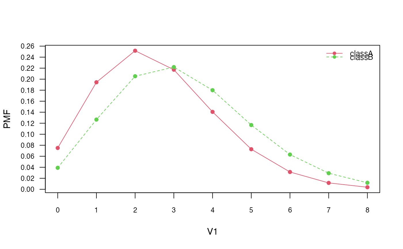
# Visualise class conditional Poisson distributions
plot(nb, "V1", prob = "conditional")
plot(pnb, which = "V1", prob = "conditional")


# Check the equivalence of the class conditional distributions
all(get_cond_dist(nb) == get_cond_dist(pnb))
#> [1] TRUE