Bernoulli Naive Bayes Classifier
bernoulli_naive_bayes.Rdbernoulli_naive_bayes is used to fit the Bernoulli Naive Bayes model in which all class conditional distributions are assumed to be Bernoulli and be independent.
Arguments
- x
matrix with numeric 0-1 predictors (matrix or dgCMatrix from Matrix package).
- y
class vector (character/factor/logical).
- prior
vector with prior probabilities of the classes. If unspecified, the class proportions for the training set are used. If present, the probabilities should be specified in the order of the factor levels.
- laplace
value used for Laplace smoothing (additive smoothing). Defaults to 0 (no Laplace smoothing).
- ...
not used.
Value
bernoulli_naive_bayes returns an object of class "bernoulli_naive_bayes" which is a list with following components:
- data
list with two components:
x(matrix with predictors) andy(class variable).- levels
character vector with values of the class variable.
- laplace
amount of Laplace smoothing (additive smoothing).
- prob1
matrix with class conditional probabilities for the value 1. Based on this matrix full probability tables can be constructed. Please, see
tablesandcoef.- prior
numeric vector with prior probabilities.
- call
the call that produced this object.
Details
This is a specialized version of the Naive Bayes classifier, in which all features take on numeric 0-1 values and class conditional probabilities are modelled with the Bernoulli distribution.
The Bernoulli Naive Bayes is available in both, naive_bayes and bernoulli_naive_bayes. The latter provides more efficient performance though. Faster calculation times come from restricting the data to a numeric 0-1 matrix and taking advantage of linear algebra operations. Sparse matrices of class "dgCMatrix" (Matrix package) are supported in order to furthermore speed up calculation times.
The bernoulli_naive_bayes and naive_bayes() are equivalent when the latter uses "0"-"1" character matrix.
The missing values (NAs) are omited while constructing probability tables. Also, the corresponding predict function excludes all NAs from the calculation of posterior probabilities (an informative warning is always given).
Author
Michal Majka, michalmajka@hotmail.com
Examples
# library(naivebayes)
### Simulate the data:
set.seed(1)
cols <- 10 ; rows <- 100 ; probs <- c("0" = 0.9, "1" = 0.1)
M <- matrix(sample(0:1, rows * cols, TRUE, probs), nrow = rows, ncol = cols)
y <- factor(sample(paste0("class", LETTERS[1:2]), rows, TRUE, prob = c(0.3,0.7)))
colnames(M) <- paste0("V", seq_len(ncol(M)))
laplace <- 0
### Train the Bernoulli Naive Bayes
bnb <- bernoulli_naive_bayes(x = M, y = y, laplace = laplace)
summary(bnb)
#>
#> ============================ Bernoulli Naive Bayes =============================
#>
#> - Call: bernoulli_naive_bayes(x = M, y = y, laplace = laplace)
#> - Laplace: 0
#> - Classes: 2
#> - Samples: 100
#> - Features: 10
#> - Prior probabilities:
#> - classA: 0.28
#> - classB: 0.72
#>
#> --------------------------------------------------------------------------------
# Classification
head(predict(bnb, newdata = M, type = "class")) # head(bnb %class% M)
#> [1] classB classB classB classB classB classB
#> Levels: classA classB
# Posterior probabilities
head(predict(bnb, newdata = M, type = "prob")) # head(bnb %prob% M)
#> classA classB
#> [1,] 0.08558455 0.9144154
#> [2,] 0.11094760 0.8890524
#> [3,] 0.19887370 0.8011263
#> [4,] 0.39836587 0.6016341
#> [5,] 0.24260388 0.7573961
#> [6,] 0.38489861 0.6151014
# Parameter estimates
coef(bnb)
#> classA:0 classA:1 classB:0 classB:1
#> V1 0.9642857 0.03571429 0.9305556 0.06944444
#> V2 0.8214286 0.17857143 0.9444444 0.05555556
#> V3 0.8571429 0.14285714 0.9027778 0.09722222
#> V4 0.8928571 0.10714286 0.8750000 0.12500000
#> V5 0.8928571 0.10714286 0.8472222 0.15277778
#> V6 0.8571429 0.14285714 0.9027778 0.09722222
#> V7 0.8571429 0.14285714 0.8888889 0.11111111
#> V8 0.9642857 0.03571429 0.8750000 0.12500000
#> V9 0.8571429 0.14285714 0.8611111 0.13888889
#> V10 0.8928571 0.10714286 0.8888889 0.11111111
### Sparse data: train the Bernoulli Naive Bayes
library(Matrix)
M_sparse <- Matrix(M, sparse = TRUE)
class(M_sparse) # dgCMatrix
#> [1] "dgCMatrix"
#> attr(,"package")
#> [1] "Matrix"
# Fit the model with sparse data
bnb_sparse <- bernoulli_naive_bayes(M_sparse, y, laplace = laplace)
# Classification
head(predict(bnb_sparse, newdata = M_sparse, type = "class"))
#> [1] classB classB classB classB classB classB
#> Levels: classA classB
# Posterior probabilities
head(predict(bnb_sparse, newdata = M_sparse, type = "prob"))
#> [,1] [,2]
#> [1,] 0.08558455 0.9144154
#> [2,] 0.11094760 0.8890524
#> [3,] 0.19887370 0.8011263
#> [4,] 0.39836587 0.6016341
#> [5,] 0.24260388 0.7573961
#> [6,] 0.38489861 0.6151014
# Parameter estimates
coef(bnb_sparse)
#> classA:0 classA:1 classB:0 classB:1
#> V1 0.9642857 0.03571429 0.9305556 0.06944444
#> V2 0.8214286 0.17857143 0.9444444 0.05555556
#> V3 0.8571429 0.14285714 0.9027778 0.09722222
#> V4 0.8928571 0.10714286 0.8750000 0.12500000
#> V5 0.8928571 0.10714286 0.8472222 0.15277778
#> V6 0.8571429 0.14285714 0.9027778 0.09722222
#> V7 0.8571429 0.14285714 0.8888889 0.11111111
#> V8 0.9642857 0.03571429 0.8750000 0.12500000
#> V9 0.8571429 0.14285714 0.8611111 0.13888889
#> V10 0.8928571 0.10714286 0.8888889 0.11111111
### Equivalent calculation with general naive_bayes function.
### (no sparse data support by naive_bayes)
# Make sure that the columns are factors with the 0-1 levels
df <- as.data.frame(lapply(as.data.frame(M), factor, levels = c(0,1)))
# sapply(df, class)
nb <- naive_bayes(df, y, laplace = laplace)
summary(nb)
#>
#> ================================= Naive Bayes ==================================
#>
#> - Call: naive_bayes.default(x = df, y = y, laplace = laplace)
#> - Laplace: 0
#> - Classes: 2
#> - Samples: 100
#> - Features: 10
#> - Conditional distributions:
#> - Bernoulli: 10
#> - Prior probabilities:
#> - classA: 0.28
#> - classB: 0.72
#>
#> --------------------------------------------------------------------------------
head(predict(nb, type = "prob"))
#> classA classB
#> [1,] 0.08558455 0.9144154
#> [2,] 0.11094760 0.8890524
#> [3,] 0.19887370 0.8011263
#> [4,] 0.39836587 0.6016341
#> [5,] 0.24260388 0.7573961
#> [6,] 0.38489861 0.6151014
# Obtain probability tables
tables(nb, which = "V1")
#> --------------------------------------------------------------------------------
#> :: V1 (Bernoulli)
#> --------------------------------------------------------------------------------
#>
#> V1 classA classB
#> 0 0.96428571 0.93055556
#> 1 0.03571429 0.06944444
#>
#> --------------------------------------------------------------------------------
tables(bnb, which = "V1")
#> --------------------------------------------------------------------------------
#> :: V1 (Bernoulli)
#> --------------------------------------------------------------------------------
#> classA classB
#> 0 0.96428571 0.93055556
#> 1 0.03571429 0.06944444
#>
#> --------------------------------------------------------------------------------
# Visualise class conditional Bernoulli distributions
plot(nb, "V1", prob = "conditional")
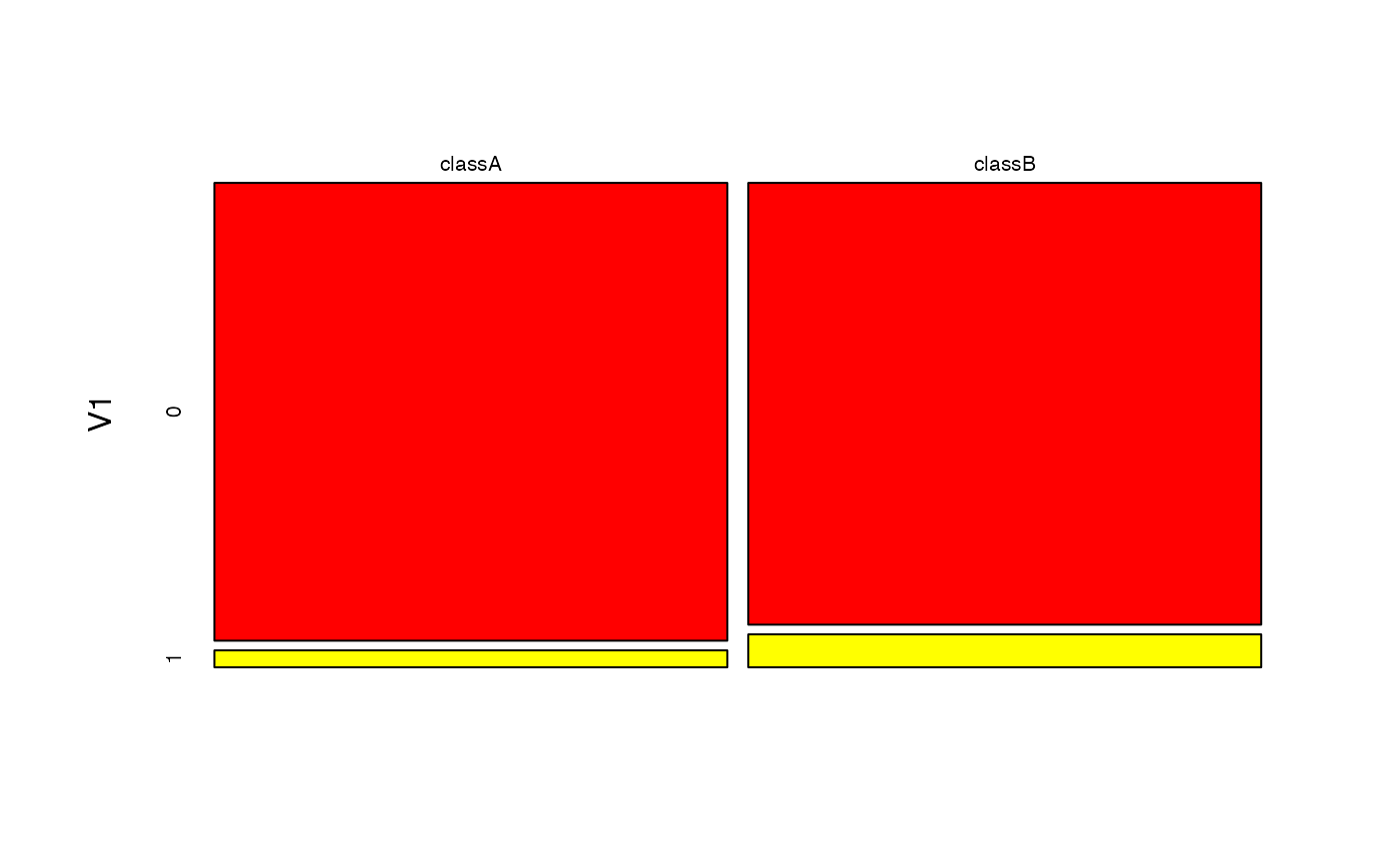 plot(bnb, which = "V1", prob = "conditional")
 # Check the equivalence of the class conditional distributions
all(get_cond_dist(nb) == get_cond_dist(bnb))
#> [1] TRUE
# Check the equivalence of the class conditional distributions
all(get_cond_dist(nb) == get_cond_dist(bnb))
#> [1] TRUE