Plot Method for bernoulli_naive_bayes Objects
plot.bernoulli_naive_bayes.RdPlot method for objects of class "bernoulli_naive_bayes" designed for a quick look at the class marginal distributions or class conditional distributions of 0-1 valued predictors.
Arguments
- x
object of class inheriting from
"bernoulli_naive_bayes".- which
variables to be plotted (all by default). This can be any valid indexing vector or vector containing names of variables.
- ask
logical; if
TRUE, the user is asked before each plot, seepar(ask=.).- arg.cat
other parameters to be passed as a named list to
mosaicplot.- prob
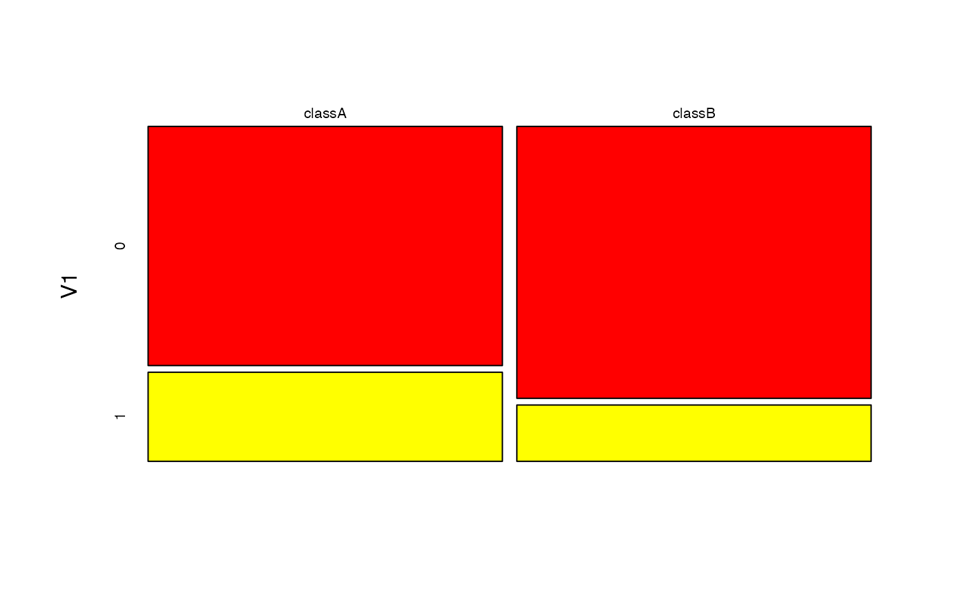
character; if "marginal" then marginal distributions of predictor variables for each class are visualised and if "conditional" then the class conditional distributions of predictor variables are depicted. By default, prob="marginal".
- ...
not used.
Details
Class conditional or class conditional distributions are visualised by mosaicplot.
The parameter prob controls the kind of probabilities to be visualized for each individual predictor \(Xi\). It can take on two values:
"marginal": \(P(Xi|class) * P(class)\)
"conditional": \(P(Xi|class)\)
Author
Michal Majka, michalmajka@hotmail.com
Examples
# Simulate data
cols <- 10 ; rows <- 100 ; probs <- c("0" = 0.4, "1" = 0.1)
M <- matrix(sample(0:1, rows * cols, TRUE, probs), nrow = rows, ncol = cols)
y <- factor(sample(paste0("class", LETTERS[1:2]), rows, TRUE, prob = c(0.3,0.7)))
colnames(M) <- paste0("V", seq_len(ncol(M)))
laplace <- 0.5
# Train the Bernoulli Naive Bayes model
bnb <- bernoulli_naive_bayes(x = M, y = y, laplace = laplace)
# Visualize class marginal probabilities corresponding to the first feature
plot(bnb, which = 1)
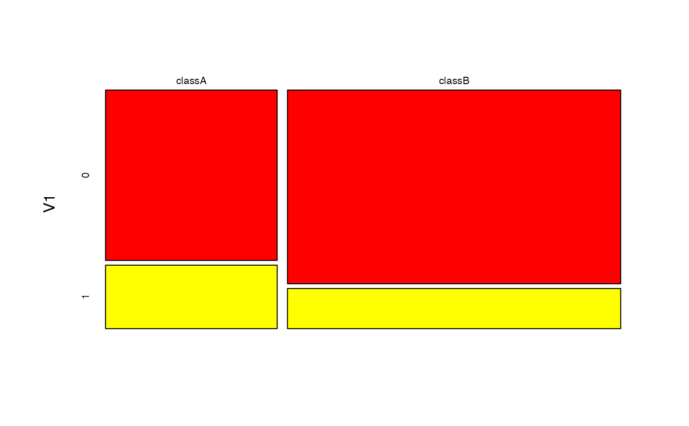 # Visualize class conditional probabilities corresponding to the first feature
plot(bnb, which = 1, prob = "conditional")
# Visualize class conditional probabilities corresponding to the first feature
plot(bnb, which = 1, prob = "conditional")